Lab #3: Non-constant acceleration

Non-Constant Acceleration

Samuel
Ellis
Mia
9-12-2016

2.

Find how far the elephant goes before coming to rest.

3.

In calculus, when we were given position function, we take derivative of the function to find its velocity or acceleration. If we were given acceleration function, we can take the integral to find the velocity and position. In this case, the mass of rocket is changing. We can use acceleration equal force divide by mass to find acceleration.  Then use that to find its position.

 4.

1. open up a new excel spreadsheet.

2. put appropriate values in for v_o and x_o.

3. set delta t to be 1 second. put in the other appropriate values in cells B1  through B4.

4. Input a formula into cell A9 that will calculate the appropriate time, and that you can fill down. Use $B$5 into your formula, so the cell will let you calculate the acceleration at any time. Fill that formula down to cell B9.

5. Input cell C9 calculate the average acceleration for that first delta t interval.

6. In cell D9 calculate the change in velocity for the first time interval.

7. In cell E9 calculate the speed at the end of that time interval.

8. In cell F9 calculate average speed at at end of time interval.

9. In cell G9 calculate the change in position of the elephant during that time interval.

10. In cell H9 calculate the position of the elephant.

11. Change the time interval from 1 second to 0.1s and see if makes a different.

12. Change the time interval to 0.05 instead of 0.1s and see if makes a different.

5. & 6 &7

( The difference between those data is the change in time interval, and the highlighted area is for time = 1, 0.5,0.01. and we got 248, 248,248)

8.

In conclusion, we had used integral to find the displacement for elephant, by putting data into excel and create bunch function. Then we change the time interval to see if it will make the different, the answer is NO.

Lab #2: Free Fall

Free Fall

Samuel
Ellis
Mia
8-31-2016

2.

To examine in the absent of all other external forces expect gravity, a falling body will accelerate at -9.8 m/s^2

3.

Theory: In physics class, we always assume gravity will be -9.8 meter per second square. In the real world, however, it doesn't always happen that way. At different location, gravity will vary from -9 meter square per second to -10 meter square per second. So in this experiment, we let gravity to be our only source of force. By letting gravity act on an object, we can determine how fast it accelerate downward. And since gravity is the only force acting on that object, the acceleration will be gravity.

 4.

1. Pull a piece of paper tape between the vertical wire and the vertical post of the device. Clip it with a weight to keep the paper "tight".

2. Turn the dial hooked up to the electromagnet up a bit.

3. Hang the wooden cylinder with the metal ring around it on the electromagnet.

4. Turn on the power on the sparker box.

5. Hold down the spark button on the sparker box.

6. Turn the electromagnet off so that the thing falls.

7. Turn off the power to the sparker thing.

8. Tear off the paper strip and set up the spark paper for the next person to get their data.

Excel:

1. select your data in columns D and E. Click on the Chart tab, then choose scatter, then Marked Scatter to give an XY (scatter) graph with the point NOT connected.

2. Use the Chart Layout tab to give appropriate titles (with unit) for your graph and your graph axes.

3. under the chart layout tab click on trendline, choose trendline option. choose a liner fit. under the options choose "display equation on chart" and "display r-squared value on charf". when you click "OK" this should give you a line and equation on the graph. Double-click on the equation on your chart. use the numbers formatting to get a reasonable number of decimal places in your answers. use the font menu to make the equation large enough that it will show up nicely when you to print or photograph your graph. 

4.Select column A and B. follow the same steps above except when you get to add trendline choose a polymonial fit of order 2.

5 & 6

(we first measure the distance between each dot(at least 14). Then input data into computer using excel, then follow the procedure above.By using linear fit, we can get an equation of the linear line. Which give up the Constance.  At the end we got speed vs time & distance vs time graph. Then we the number we got in the graph, which is 901 as our gravity Constance.

(this is the data from other groups)

8.

At the end, our calculation shows that gravity for our experiment is around 9 meter per second square. Which is lay between 9 and 10, so its normal. Gravity constance vary at different location. In conclusion, we find the acceleration of gravity by using the distance between dots and know the punch time for each dots. Then plot those data using excel and use linear fit to find gravity. 

Lab#6: Propagated Uncertainty in Measurements

Propagated Uncertainty in Measurements

Samuel
Ellis
Mia
9-7-2016

2.

Every experiment have its little error, to avoid these error we have to get a more precise equipment. Or we can use uncertainty measurement to find the error range so we can know what value is our answer lay between.

3. 

To use propagated uncertainty, we first have to know what +- the measurement lay between and we also need to know how to take partial derivative. To calculate uncertainty, we have to find the answer without using uncertainty and then take a square root of double uncertainty(^2), so we get a constant value.

4.

1. Watch lecture online in Moodlerooms about propagated uncertainty.
2. weight metals
3. Measure two different metals using calipers.
4. Determine it uncertainty and record your data.
5. Calculate uncertainty using above data.

5.

We were given two cylindrical shapes metal but in different material and length. Longer one is aluminum and shorter one is iron.(measurement below) 

6.

 we got an equation using square root of doubling everything to get uncertainty for metals. 2nd picture is uncertainty for aluminum. 

7. 

8.

The more accurate we want our data to be, we either need to get more precise measuring tool or use propagated uncertainty to the how much error is our actual answer differ from the most accurate one.
By taking partial derivative, we can find uncertainty.  

Lab #4: Modeling the fall of an object falling with air resistance

Air Resistance

Samuel
Ellis
Mia
9-19-2016

2. 

We have an expectation that air resistance force on a particular object depends on the object's speed, its shape, and the material it is moving through. We can model this expectation as a power law. 

3.

Power law = F_resistance = kv^n. k is constant(shape of object density of air), v is speed. To determine a falling object, we need to know it speed and exponent and base on those data we can find air resistance. 

4.

  1. Turn on LoggerPro, open "video capture" 

  2. Capture video for 1,2,3,4, and 5 coffee filter falling from balcony.

  3. Get terminal velocities for each one by fitting the linear portion of the position vs time graph for each.

  4. Plot your data appropriately to determine values for k and n. 

  5. In excel worksheet, label t, a, delta v, and v.
  6. Set t = 1/30 of a second
  7. Once you have calculate columns in excel for v and x as function of times, determine what your model predicts for the terminal velocity of the various coffee filter. 

  

5. 

150 coffee filters = 134.2g

1 coffee filter = 0.895g

Slope

1= 1.537

2=   2.28

3=   2.74

4=   3.33

5=    4.10

A= 0.00419+- 0.005

B= 1.777+- 0.1179

6.

 (Then we input different mass of coffee filter to get air resistance force)

(Find in what time does velocity stop increasing) 

7.

  

Above, is the speed vs air force graph. We inputted the speed of coffee filter(s) from 5 different weights along with their air-resistance force. And then used "power fit" curve to find the equation of the curve, which turn out to be k= 0.00419+- 0.0005 and n= 1.777+-0.1139. 

8.

At the end, we generate an equation for air-resistance force acting on coffee filter. Air-resistance force increase as velocity increase. We first determine filters speed by video taping it falling speed, then used 1 meter ruler in the video for reference distance so we can plot point as every 1/30 of a second. So we find our speed and time, we just need to use power fit to find its equation. 

Lab 5: Trajectories

Trajectories

Samuel
Ellis
Mia
9-14-2016

2.

To use your understanding of projectile motion to predict the impact point of a ball on an inclined board and compare it with actual distance.

3.  

 We first assume there will be no frictional force and air-resistance, and gravity will be -9.8m/s^2. Then we are allow to use our kinematic equation to solve for time , distance and velocity for both x and y direction. 

4. 

Material: Aluminum "v-channel", steel ball, board, ring stand, clamp, paper, carbon paper

1. Launch the ball from a readily identifiable and repeatable point near the top of the inclined ramp. Notice where it hits the floor.

2. Tape a piece of carbon paper to the floor around where the ball landed. Launch the ball five times from the same place as before and verify the same place each time.

3. Determine the height of the bottom of the ball when it launches, and how far out from the table's edge it landed. 

4. Determine the launch speed of the ball from your measurements. Sketch the dimensions clearly.

5. Derive an expression that would allow you to determine the value of d given that you know v_o and theta. 

6. Place a board such that it touches the end of the lab table and the floor. Put a heavy mass on the floor at the foot of the board and use duct tap to fix the mass in place. Attach a piece of carbon paper to your board such that it "surrounds" the spot where you expect your ball to land. Make appropriate measurement, launching your ball five times from the same spot.

7. Determine the experimental value of your landing distances d and report your experimental value as d

8. Compare your experimental and theoretical values for d.  

(This is the spot where ball landed(darker one))

5. & 6.

( we first use y=1/2*a*t^2, to find the time in the air, then use x=v*t to solve for the velocity)

(Then we derived an equation base on x and y direction to solve for distance)

7.

Does not require graph.

8.

d=(2*(1.8^2)*sin(26))/(9.8*cos(26)^2)= 0.359m. At the end, we found the distance from releasing the ball to where it landed. During the process, we have to combined both x and y direction. So we can determine the distance from its air time and the horizontal speed.  

Lab #7: Modeling Friction Forces

Modeling Friction Forces

Samuel
Ellis
Mia
9-21-2016

2. 

In this experiment, we tried to record data when perform some friction related experiments, and uses those data to calculate frictional force acting between object and surface

3. 

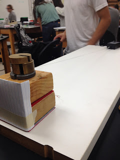
Theory: 1. Static frictions is the force acting between two bodies when they are not moving relative to one another. We tried to find the minimum static friction force that move object. If we place weights slowly and cautiously, then right before object is moving, that will be the minimum static force. Since the movement of an object require overcome static force, in this way we can know the minimum  force to overcome static force.
                 2. Kinetic friction as being proportional to the normal force, and independent of the area of the moving object. We used force sensor apply with constant force to collect data that that opposite force. In this case, it will be the kinetic friction force. 

4.

(1)

    1. Place the felt-side of the block on the lab table. Ties a string to the block and over a pulley at the end of the table.

    2. Patiently and slowly add weight to hanging weights. 

    3. Until block start sliding, remove the last weight you added.

    4. Record your data and repeat same procedure but with different mass of block.

    (2)
    1. Plug in a LabPro and connect it to computer with USB cable. Plug force sensor and switch it to 10-N range
    2. Weight the wooden block.
    3. Calibrate the force sensor using 500-grams hanging mess.
    4. Hold force sensor horizontally and zero the force sensor.
    5. Tie a string between force sensor and block. Click "Collect" and slowly pull force sensor horizontally.
    6. Repeat same procedure, but with different mass of block.

    (3) 

     1. Place a block on a horizontal surface.
     2. Slowly raise one end of the surface, tilting it until the block starts to slip.
     3. Use the angle at witch slipping just begin 

   (4)
    1. With motion detector at the top of an incline steep enough that a block will accelerate down the incline

    2. Measure the angle of the incline and the accelerate of the block.
    3. Determine the kinetic friction between block and surface from your measurement.

   5. & 6.

   (1)

    (2)

    m(block)          Kinetic Friction

    1. 180g             0.5507
    2. 320g             0.8970
    3. 520g             1.48
    4. 720g             2.13

   

    (3)

   

   (4)

   

  (5)

7. 

After we got our data from mass of the block and kinetic friction, we begin plug those number into LoggerPro. And used proportion fit to find the coefficient of kinetic friction. And we got 0.299+- .004. 

Since we placed block(s) on the incline plane and used motion detector to record data. We got position vs time & velocity vs time graph. And we highlight the area when the block start moving, then we use linear fit to velocity vs time to find its slope. And we got 1.462m/s.

8. 

The calculation from our data did not quite match with the data from computer. For instance, #4 we got 0.222 for kinetic friction. However, we received 0.2999 from LoggerPro. The reason for the difference is because maybe there have air-resistance or due to unbalance pull from people. And for #5, we got 1.81 from calculation. However, it show 1.46 in LoggerPro. The difference might due to adding of weights. Maybe because when we added weighs, we "drop" them too hard, which cause additional force to act on downward acceleration. 

Lab#1

1. Finding a relationship between mass and period for an inertial balance, Elis and Mia, 8-29-2016
2. To find relationship between period and mass for inertial pendulum.
3. Theory: Model relationship as T:A(m+Mtray)^n
                  If we are able to find the relationship between time and period, then we are able to determine mass by calculating its oscillation.
4. Procedure: Metal tray, clamped to table, tape to the end, pass through photogate measure period. Add 0g to 800g to tray(100 at a time), measure period each time.
5.

6. 

7. We measured  the period of oscillation for calculator and phone, it came out to be 0.833s for calculator and 0.4206s for phone. And I plotted the number into the equation above, it came out near to it actual weight, which is 221g and 167g.

8. We were able to determine object's weight based its period of oscillation. Even though the number does not came out to be exact mass, due to human error or machine delay.